728x90

이 글은 양주종의 코딩스쿨 리눅스(Linux) 기초 강좌 30강 모음 수강하며 정리한 글입니다.


11강 디렉토리 구조

(일반 사용자 id: j, pw: j)

(관리자 id: root, pw: r)


[j@hj0216 ~]$ ll /
합계 20
drwxr-xr-x.   2 root root    6  1월 15 21:25 ace
lrwxrwxrwx.   1 root root    7  1월 15 19:04 bin -> usr/bin
dr-xr-xr-x.   5 root root 4096  1월 15 19:15 boot
drwxr-xr-x.  19 root root 3040  1월 24 21:42 dev
drwxr-xr-x.  74 root root 8192  1월 24 21:42 etc
drwxr-xr-x.   3 root root   15  1월 15 19:13 home
lrwxrwxrwx.   1 root root    7  1월 15 19:04 lib -> usr/lib
lrwxrwxrwx.   1 root root    9  1월 15 19:04 lib64 -> usr/lib64
drwxr-xr-x.   2 root root    6  4월 11  2018 media
drwxr-xr-x.   2 root root    6  4월 11  2018 mnt
drwxr-xr-x.   2 root root    6  4월 11  2018 opt
dr-xr-xr-x. 105 root root    0  1월 24 21:42 proc
dr-xr-x---.   3 root root  147  1월 15 20:08 root
drwxr-xr-x.  24 root root  740  1월 24 21:42 run
lrwxrwxrwx.   1 root root    8  1월 15 19:04 sbin -> usr/sbin
drwxr-xr-x.   2 root root    6  4월 11  2018 srv
dr-xr-xr-x.  13 root root    0  1월 24 21:42 sys
drwxrwxrwt.  10 root root 4096  1월 24 21:43 tmp
drwxr-xr-x.  13 root root  155  1월 15 19:04 usr
drwxr-xr-x.  19 root root  267  1월 15 19:16 var

ll /

/: 최상위(root) dir

ace/: 

bin@: 일반 사용자들이 사용하는 명령어들이 모인 dir을 가르키는 soft link

boot/: 부팅에 필요한 정보를 가진 파일들이 있는 dir

dev/: device, 장치 파일(키보드, 모니터 등)과 관련된 dir (물리적 장치가 파일화되어 저장)

etc/: 시스템 설정과 관련된 dir

home/: 일반 사용자 home dir이 생성되는 dir (사용자 추가 시, 사용자 id와 동일한 dir이 이곳에 자동 생성)

lib@: library, 시스템 부팅이나 bin, sbin dir에 있는 binary file 실행에 필요한 공유 lib dir

lib64@: 시스템 부팅이나 bin, sbin dir에 있는 binary file 실행에 필요한 공유 lib dir

media/: USB 등의 외부 장치들의 파운트 포인트(연결)로 사용되는 dir (OS에서 자동으로 마운팅해주는 포인트로 주로 사용)

mnt/: mount, USB 등의 외부 장치들의 파운트 포인트(연결)로 사용되는 dir (사용자가 직접 마운트하는 경로로 사용)

opt/: optional, 추가 응용프로그램 pkg 설치가 되는 dir

proc/: process, 현재 메모리에 존재하는 작업들이 파일형태로 존재하는 dir

root/: root의 home dir

run/: 현재 실행중인 process가 저장되는 dir

sbin@: super user bin, 시스템 관리자들이 사용하는 명령어들이 모인 dir을 가르키는 soft link

srv/: served, 다른 시스템에게 제공되는 파일들이 모여있는 dir

sys/: 리눅스 커널 관련 정보가 있는 dir

tmp/: 임시 dir, 일반 사용자들이 home dir 이외 접근할 수 있는 유일한 dir, 시스템 운영 중 발생한 임시 데이터 저장(부팅 시 초기화), 스티키 비트(sticky bit)* 설정

usr/: unix system resource, 일반 사용자들을 위한 대부분의 프로그램 lib 파일들이 위치해 있는 dir로 window의 program files과 유사

var/: variable, 가변 dir로 시스템 운영중 발생한 데이터와 작동 기록(log)이 저장되는 dir


* sticky bit(공유 모드): sticky bit가 설정된 dir에서는 모든 사용자가 파일이나 dir을 만들 수는 있지만, 파일 또는 dir의 소유주나 슈퍼 유저만 삭제, 변경을 할 수 있음


참고 자료

📑 [리눅스, Linux] 디렉토리(directory) 구조

📑 [LINUX] 📚 리눅스 디렉토리 구조 - 한눈에 정리

📑 디렉토리와 파일 시스템

📑 sTicky Bit (스티키비트) SetUD / SetGD


728x90
728x90

이 글은 뉴렉쳐 오라클 데이터베이스 SQL 강의 수강하며 정리한 글입니다.


02강 - 오라클 DBMS 18c XE 설치하기


2023 ver.
1. oracle site 회원가입
2. Developers - Developer Resource Center
3. DownLoad - DataBase
4. DataBase Express Edition
5. Prior Release Archive
6. Oracle DataBase 18c Express Edition for Windows x64
7. setup.exe “관리자 권한으로 실행”

 * 설치 중 Oracle DataBase 정보: PW -> 향후 oracle DB 접속 시 사용할 PW


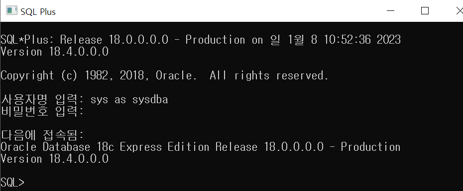
Oracle DBMS는 server program으로 사용자가 server program에 접근할 수 있도록 하는 사용자 interface인 client program이 필요
→ Oracle에서는 client program으로 consol 기반의 SQL Plus / window 기반의 SQL developer의 utility 제공
→ client program을 통해서 사용자로부터 정보를 입력받아 server program과 통신하여 실행하고 그 결과를 사용자에게 보여줌


SQL plus 실행 및 접속

1. SQL Plus 실행
2. sys as sysdba 입력 및 설치 시, 설정한 비밀번호 입력


참고 자료

📑 [Database] 오라클 설치와 기본 사용방법(SQL Plus, 최신 버전 SQL Developer)


소스 코드

🔗 HJ0216/TIL/OracleSQL

728x90
728x90

기본 환경: IDE: VS code, Language: Python


1. Save model and weights

# save_model_and_weights.py

import numpy as np

from sklearn.datasets import load_boston
from sklearn.model_selection import train_test_split
from sklearn.preprocessing import MinMaxScaler, StandardScaler
from sklearn.metrics import mean_squared_error, r2_score

from tensorflow.keras.models import Model
from tensorflow.keras.layers import Dense, Input
from tensorflow.keras.callbacks import EarlyStopping

# Model save
path = './_save/' # ./ 현재(STUDY) dir
# path = '../_save/' # ../ 상위 dir
# path = 'c:/study/_save/' # 경로 대소문자 구분 X


# 1. Data
dataset = load_boston()
x = dataset.data # for training
y = dataset.target # for predict

x_train, x_test, y_train, y_test = train_test_split(
    x, y,
    train_size=0.7,
    random_state=123
)

scaler = MinMaxScaler()
scaler.fit(x_train)
x_train = scaler.transform(x_train)
x_test = scaler.transform(x_test)


# 2. Model(Function)
input1 = Input(shape=(13,))
dense1 = Dense(64, activation='relu')(input1)
dense2 = Dense(32, activation='relu')(dense1)
output1 = Dense(1, activation='linear')(dense2)
model = Model(inputs=input1, outputs=output1)

# save model before training
model.save(path+'save_model1.h5')
# save weights before training(훈련이 되지 않은 가중치이므로 사용X)
model.save_weights(path +'save_weights1.h5')

# 3. compile and train
model.compile(loss='mse', optimizer='adam', metrics=['mae'])
earlyStopping = EarlyStopping(monitor='val_loss', mode='min', patience=32, restore_best_weights=True, verbose=1)
hist = model.fit(x_train, y_train,
          epochs=512,
          batch_size=16,
          validation_split=0.2,
          callbacks=[earlyStopping],
          verbose=1)

# save model and weight after training
model.save(path+'save_model2.h5')
# save weights after training
model.save_weights(path+'save_weights2.h5')


# 4. evaluate and predict
loss = model.evaluate(x_test, y_test)
y_predict = model.predict(x_test)

def RMSE (y_test, y_predict):
    return np.sqrt(mean_squared_error(y_test, y_predict))
print("RMSE: ", RMSE(y_test, y_predict))

r2 = r2_score(y_test, y_predict)
print("R2: ", r2)


'''
Result
RMSE:  4.122959900727362
R2:  0.7896919500228364

'''

* 훈련 전

- model.save(path+'save_model1.h5')

: model 및 weights 저장

: ⚠️ 훈련 전이므로 저장된 weights는 사용 X
- model.save_weights(path +'save_weights1.h5')

: weights 저장

: ⚠️ 훈련 전이므로 저장된 weights는 사용 X


** 훈련 후

- model.save(path+'save_model2.h5')

: model 및 weights 저장

model.save_weights(path+'save_weights2.h5')

: weights 저장


2. Load model and weights

# load_model_and_weights.py

import numpy as np

from sklearn.datasets import load_boston
from sklearn.model_selection import train_test_split
from sklearn.preprocessing import MinMaxScaler, StandardScaler
from sklearn.metrics import mean_squared_error, r2_score

from tensorflow.keras.models import Sequential, Model, load_model
from tensorflow.keras.layers import Dense, Input

# saved model path
path = './_save/' # ./ 현재(STUDY) dir
# path = '../_save/' # ../ 상위 dir
# path = 'c:/study/_save/' # 경로 대소문자 구분 X


# 1. Data
dataset = load_boston()
x = dataset.data # for training
y = dataset.target # for predict

x_train, x_test, y_train, y_test = train_test_split(
    x, y,
    train_size=0.7,
    random_state=123
)

# scaler = StandardScaler()
scaler = MinMaxScaler()
scaler.fit(x_train)
x_train = scaler.transform(x_train)
x_test = scaler.transform(x_test)


# 2. Model(Function)
model = load_model(path+'save_model1.h5')
# save_model1.h5와 동일한 모델 구성 반환
# Model Construction 생략 가능


# 3. compile and train
model = load_model(path + 'save_model2.h5')
# save_model2.h5와 동일한 모델 구성 및 가중치 반환
# Model construction, compile and train 생략 가능


# 4. evaluate and predict
loss = model.evaluate(x_test, y_test)
y_predict = model.predict(x_test)

def RMSE (y_test, y_predict):
    return np.sqrt(mean_squared_error(y_test, y_predict))
print("RMSE: ", RMSE(y_test, y_predict))

r2 = r2_score(y_test, y_predict)
print("R2: ", r2)


'''
Result
RMSE:  4.122959900727362
R2:  0.7896919500228364

'''

* 훈련 전

- model = load_model(path+'save_model1.h5')

: 저장된 model 및 weights 불러오기

⚠️ 훈련 전이므로 저장된 weights는 무의미
- model.load_weights(path + 'save_weights1.h5')

: 저장된 weights 불러오기

⚠️ weights를 가져왔으므로 fit 필요없으나, 훈련 전 저장된 weights 무의미


** 훈련 후

- model = load_model(path + 'save_model2.h5')

: 저장된 model 및 weights 불러오기

- model.load_weights(path + 'save_weights2.h5')

: 저장된 weights 불러오기

⚠️ RuntimeError: You must compile your model before training/testing. Use `model.compile(optimizer, loss)`.
⚠️ 가중치만 저장(Model 및 Compile 저장 X) -> 모델 구성 후 compile 필요


➕ weight만 따로 save 하는 이유
→ 큰 모델의 모델 및 가중치 저장 시, 파일의 크기가 큼(불러오기에서 문제가 발생할 가능성 존재)

 사이즈가 상대적으로 작은 훈련 결과 가중치만 저장하여 안전하게 불러오기


파일 확장자 .h5와 .hdf5

.h5 = .hdf5

HDF5는 Hierarchical Data Format이며 self-describing이 되는 고성능 데이터포맷 또는 DB 

HDF5 파일을 생성하면 먼저 /라는 루트 그룹이 생성되고 그 하위에 트리 구조로 다른 그룹을 생성할 수 있음

그룹 하위에 다른 그룹이 있을 수도 있고, 데이터셋이 존재할 수도 있으며 운영체계의 디렉토리-파일 구조와 일치 


소스 코드

🔗 HJ0216/TIL


참고 자료

📑 7.1 HDF5의 특징


728x90
728x90

기본 환경: IDE: VS code, Language: Python


CNN(Convolution Neural Network, 합성곱 신경망)

: 영상처리에 많이 활용되는 합성곱을 사용하는 신경망 구조

기존처럼 데이터에서 지식을 추출해 학습하는 것이 아니라 데이터의 특징을 추출하여 특징들의 패턴을 파악하는 구조


CNN 학습 과정
0(y) = imageA (x)

1. colvolution 과정을 통해 특성맵 추출

➕ 필요할 경우, 패딩(Padding, 결과 값 행렬의 크기를 조정하기 위해 입력 배열의 둘레를 확장하고 0으로 채우는 연산) 진행


2. Pooling 과정을 통해 데이터의 특성 강조


풀링(Pooling): 일정 크기의 블록을 통합하여 하나의 대표값으로 대체하는 연산으로 컨볼루션 층에서 출력된 특징 지도를 압축하여 특정 데이터를 강조하는 역할


3. Conv와 Pooling의 반복 연산을 통해 입력 이미지 배열을 특징들만을 포함한 하나의 1차원 배열 데이터로 변환


4. 다층 퍼셉트론 층(Fully Connected Layer)을 통한 연산 수행 및 회귀 혹은 분류 진행


CNN 기본 모델 Summary

# conv2D_model_summary

from tensorflow.keras.models import Sequential
from tensorflow.keras.layers import Dense, Conv2D, Flatten
# 이미지 = 2차원(2D) -> Conv2D 사용

model = Sequential()
# 입력: 데이터개수(무시), 가로(5), 세로(5), 색깔(1 or 3)
# 데이터의 개수는 중요하지 않으므로 (NaN, 5, 5, 1)
model.add(Conv2D(filters=10, kernel_size=(2,2),
                 input_shape=(5,5,1)))
# 이미지 픽셀 수(5*5) 1개(흑백) 3개(컬러RPG)
# kernel_size = 합을 연산할 이미지 블럭의 사이즈(2*2)
# 1 layer 연산 후 5*5 -> 4*4 -> ... 연산량이 점점 줄어감
# filter = 10: 5*5 흑백 이미지 1장을 10장으로 늘림
# hyper-parameter tuning: filters, kernel_size, activation 등

model.add(Conv2D(5, (2,2))) # model.add(Conv2D(filters=5, kernel_size=(2,2)))
# 2번째 conv2D는 1번째 모델의 output(4*4*10)
# filter = 5: 4*4(블럭화 후 이미지 크기가 줄어듬) 흑백 이미지 1장을 5장을 쌓아둠
# filter: Dense의 hidden output layer
# 이미지를 수치화하기 위해 column을 class화 하여 y값과 연결: Conv2D->Flatten
model.add(Flatten()) # (3*3*5) -> (45, ) (Nan, 45)
# column화 시키기(3*3*5=45): 45개의 특성(Column)을 갖는 n개의 이미지로 DNN 교육

model.add(Dense(units=10))
# (임의) hidden 10 layer 처리
model.add(Dense(1)) # 이미지의 최종 수치화, (Nan, 1)
# Nan = 고정적으로 제공되는 Data의 양

model.summary()
'''
Model: "sequential"
_________________________________________________________________
 Layer (type)                Output Shape              Param #
=================================================================
 conv2d (Conv2D)             (None, 4, 4, 10)          50 
                             연산에 따라 사이즈가 줄어감
 conv2d_1 (Conv2D)           (None, 3, 3, 5)           205
                              5 = filter 수
-------------------------------DNN---------------------------------
 flatten (Flatten)           (None, 45)                0 (flatten은 펴주는 것이므로 연산량 X) 

 dense (Dense)               (None, 10)                460 (bias +1)

 dense_1 (Dense)             (None, 1)                 11
 =================================================================

Conv2D parm 연산법

Param #
Conv2D 1번째: 필터 크기(kernel_size)*입력 채널(color)*출력 채널(filter)+출력 채널의 bias(filter)
-> (2*2) * 1 * 10 + 10
Conv2D 2번째: 필터 크기(kernel_size)*입력 채널(이전 filter)*출력 채널(filter)+출력 채널의 bias(filter)
-> (2*2) * 10 * 5 + 5

'''


'''
Conv2D Input_shape(rows, cols, channels)
1. rows: 행
2. columns: 열
3. channnels: color(흑백-1, 컬러-3)
-> data 개수가 x개 일 때,
(x, rows, cols, channels) 표기하는 것이 맞지만 데이터 수는 결정되어있는 상태이므로 (rows, cols, channels)로 표시

Dense Input_shape(None, cols)
-> data 개수가 x개 일 때,
(x, cols) 표기하는 것이 맞지만 데이터 수는 결정되어있는 상태이므로 (cols,)로 표시

'''


➕ Conv2D()와 Desne() Layer 정의

#Conv2D
'''
def __init__(self,
             filters, # 합성곱에 사용되는 필터의 개수
             kernel_size, # 합성곱에 사용되는 필터의 크기
             strides=(1, 1), # 풀링 필터를 이동시키는 간격, 지정해주지 않을 경우(None)에 오버랩없이 풀링 진행
             padding='valid', # conv 후 이미지 크기 유지시킬 것인지 유무
             data_format=None,
             dilation_rate=(1, 1),
             groups=1,
             activation=None, # 활성화 함수
             use_bias=True,
             kernel_initializer='glorot_uniform',
             bias_initializer='zeros',
             kernel_regularizer=None,
             bias_regularizer=None,
             activity_regularizer=None,
             kernel_constraint=None,
             bias_constraint=None,
             **kwargs): # keyword args의 줄임말
'''


#Dense
'''
def __init__(self,
             units, # 다음에 전달될 layer
             activation=None, # 활성화 함수
             use_bias=True,
             kernel_initializer='glorot_uniform',
             bias_initializer='zeros',
             kernel_regularizer=None,
             bias_regularizer=None,
             activity_regularizer=None,
             kernel_constraint=None,
             bias_constraint=None,
             **kwargs):
'''


1. Mnist dataset CNN model construction

# cnn_mnist.py

import numpy as np
import datetime

from tensorflow.keras.datasets import mnist
# mnist: 고등학생과 미국 인구조사국 직원들이 손으로 쓴 70,000개의 작은 숫자 이미지들의 집합
from tensorflow.keras.models import Sequential
from tensorflow.keras.layers import Conv2D, Flatten, Dense, Dropout
from tensorflow.keras.callbacks import EarlyStopping, ModelCheckpoint

filepath = './_save/MCP/'
filename = '{epoch:04d}-{val_loss:.4f}.hdf5'
# 04d: 10진수 빈자리 0 표시
# .4f: 소수점 4번째자리까지 표시


# 1. data
(x_train, y_train), (x_test, y_test) = mnist.load_data()
print(x_train.shape, y_train.shape)
# (60000, 28, 28) (60000,)
# 행(28), 열(28), 흑백(1-생략)인 이미지 데이터 60000개
# scalar=1인 데이터 60000개
print(x_test.shape, y_test.shape)
'''
reshpae
CNN Conv2D 처리하기 위해 4D(Tensor)화
(60000, 28, 28) -> (60000, 28, 28, 1)
'''

x_train = x_train.reshape(60000, 28, 28, 1)
x_test = x_test.reshape(10000, 28, 28, 1)

# train, test 분리되어있으므로 split 필요 X

print(np.unique(y_train, return_counts=True))
'''
y_train 다중 분류인지 데이터 특성 파악
(array([0, 1, 2, 3, 4, 5, 6, 7, 8, 9], dtype=uint8), # y_calss
array([5923, 6742, 5958, 6131, 5842, 5421, 5918, 6265, 5851, 5949], dtype=int64) y_class의 개수)
'''

'''
scaler = StandardScaler()
scaler.fit(x_train)
x_train = scaler.transform(x_train)
x_test = scaler.transform(x_test)

ValueError: Found array with dim 4.
StandardScaler expected <= 2.
StandardScaler, MinMaxScaler는 dim=2인 경우에 가능
'''


# 2. Model
model = Sequential()
model.add(Conv2D(filters=128,
                 kernel_size=(2, 2),
                 input_shape=(28, 28, 1),
                 activation='relu')) # Conv2D 후, result (27, 27, 128)
model.add(Conv2D(filters=64,
                 kernel_size=(2, 2))) # Conv2D 후, result (26, 26, 64)
model.add(Conv2D(filters=64,
                 kernel_size=(2, 2))) # Conv2D 후, result (25, 25, 64)
model.add(Flatten()) # input_dim=25*25*64=40000 = column
model.add(Dense(32, activation='relu'))  # 32- 임의
# 60000=batch_size(총 훈련 필요 대상), 40000=input_dim
model.add(Dropout(0.3))
model.add(Dense(10, activation='softmax')) # 10=y_class


# 3. Compile and train
model.compile(loss='sparse_categorical_crossentropy', optimizer='adam', metrics=['acc'])
# one-hot encoding 안했으므로, sparse
# one-hot encoding 후 (60000, 10=y_class)

earlyStopping = EarlyStopping(monitor='val_loss', mode='min', patience=32, restore_best_weights=True, verbose=1)

date = datetime.datetime.now()
date = date.strftime("%m%d_%H%M") #mmdd_hhmm

modelCheckPoint = ModelCheckpoint(monitor='val_loss', mode='auto', verbose=1,
                                   save_best_only=True,
                                   filepath=filepath + 'cnn_mnist_' + date + '_' + filename)


model.fit(x_train, y_train, epochs=64, batch_size=512,
                    validation_split=0.2,
                    callbacks=[earlyStopping, modelCheckPoint],
                    verbose=1)


# 4. evaluate and predict
result = model.evaluate(x_test, y_test)
print("loss: ", result[0])
print("acc: ", result[1])


'''
Result
loss:  0.16762535274028778
acc:  0.9696000218391418

'''


2. Cifar10 dataset CNN model construction

# cnn_cifar10.py

import datetime
import numpy as np

from tensorflow.keras.datasets import cifar10, cifar100
# cifar10: 총 10개의 label, label 당 6000개의 이미지로 이뤄진 data set
from tensorflow.keras.models import Sequential
from tensorflow.keras.layers import Conv2D, Flatten, Dense, Dropout, MaxPooling2D
from tensorflow.keras.callbacks import EarlyStopping, ModelCheckpoint

filepath = './_save/MCP/'
filename = '{epoch:04d}-{val_loss:.4f}.hdf5'


# 1. data
(x_train, y_train), (x_test, y_test) = cifar10.load_data()
print(x_train.shape, y_train.shape) # (50000, 32, 32, 3) (50000, 1)
print(x_test.shape, y_test.shape) # (10000, 32, 32, 3) (10000, 1)

# pixel값의 최대 수치인 255로 직접 나눠주어 정규화 scaling
x_train = x_train/255
x_test = x_test/255

print(np.unique(y_train, return_counts=True))
'''
(array([0, 1, 2, 3, 4, 5, 6, 7, 8, 9], dtype=uint8),
 array([5000, 5000, 5000, 5000, 5000, 5000, 5000, 5000, 5000, 5000], dtype=int64))
'''


# 2. Model
model = Sequential()
model.add(Conv2D(filters=128,
                 kernel_size=(2, 2),
                 padding='same',
                 input_shape=(32, 32, 3),
                 activation='relu'))
model.add(MaxPooling2D((2, 2)))
model.add(Conv2D(filters=64,
                 kernel_size=(2, 2),
                 padding='same',
                 activation='relu'))
model.add(MaxPooling2D((2, 2)))
model.add(Conv2D(filters=64,
                 kernel_size=(2, 2),
                 padding='same',
                 activation='relu'))
model.add(Flatten())
model.add(Dense(32, activation='relu'))
model.add(Dropout(0.5))
# dropout = rate: Float between 0 and 1. Fraction of the input units to drop.
# 사용하지 않을 node의 비율
model.add(Dense(10, activation='softmax'))


# 3. Compile and train
model.compile(loss='sparse_categorical_crossentropy', optimizer='adam', metrics=['acc'])

earlyStopping = EarlyStopping(monitor='val_loss', mode='min', patience=32, restore_best_weights=True, verbose=1)

date = datetime.datetime.now()
date = date.strftime("%m%d_%H%M")

modelCheckPoint = ModelCheckpoint(monitor='val_loss', mode='auto', verbose=1,
                                   save_best_only=True,
                                   filepath=filepath + 'cnn_cifar10_' + date + '_' + filename)

model.fit(x_train, y_train, epochs=256, batch_size=128,
                    validation_split=0.2,
                    callbacks=[earlyStopping, modelCheckPoint],
                    verbose=1)


# 4. evaluate and predict
result = model.evaluate(x_test, y_test)
print("loss: ", result[0])
print("acc: ", result[1])


'''
Result
loss:  0.9623041749000549
acc:  0.6858000159263611

'''


MinMaxScaler, StandardScaler Dimension Error 해결

# cnn_mnist_scaler.py

import numpy as np

from sklearn.preprocessing import StandardScaler

from tensorflow.keras.datasets import mnist, cifar10, cifar100
from tensorflow.keras.models import Sequential
from tensorflow.keras.layers import Conv2D, Flatten, Dense, Dropout
from tensorflow.keras.callbacks import EarlyStopping, ModelCheckpoint


# 1. data
(x_train, y_train), (x_test, y_test) = mnist.load_data()
# x_train.shape: (60000, 28, 28)
# x_test.shape: (10000, 28, 28)
print(x_train.shape, x_test.shape)
x_train = x_train.reshape(60000, 784)
x_test = x_test.reshape(10000, 784)

scaler = StandardScaler()
scaler.fit(x_train)
x_train = scaler.transform(x_train)
x_test = scaler.transform(x_test)

'''
ValueError: Found array with dim 4.
StandardScaler expected <= 2.
StandardScaler, MinMaxScaler는 dim=2인 경우에 가능
'''
x_train = x_train.reshape(60000, 28, 28, 1)
x_test = x_test.reshape(10000, 28, 28, 1)
# dimension을 변경했을 경우, 내부적인 수치는 성능에 따라 변경 가능
# (60000, 784) -> (60000, 28, 28, 1) O (60000, 14, 56, 1) O ...


➕ CNN Model과 HyperParameterTuning

# 2. Model
model = Sequential()
model.add(Conv2D(filters=128,
                 kernel_size=(3, 3),
                 strides=1,
                 padding='same',
                 input_shape=(28, 28, 1),
                 activation='relu'))
'''
# padding
padding=valid
output_shape=(26,26,128)
output shape = input_shape - kernel_size +1 (Not using padding)
padding=same
output_shape=(28,28,128)

'''

1. filters: 훈련할 이미지의 개수

2. kernel_size: feature map 크기 결정

3. strides: data 중복 관리

4. padding opt: data 손실 관리

5. activation: 모델의 표현력 향상, 모델의 비선형성


소스 코드

🔗 HJ0216/TIL


참고 자료

📑 딥러닝 #2 (CNN 구조, CNN 학습 알고리즘)

📑 CNN 파라미터 숫자 계산

📑 [딥러닝 첫걸음]간단한 모델 만들기

📑 FUNDAMENTAL 29. 활성화 함수의 이해


728x90
728x90

기본 환경: IDE: VS code, Language: Python


⭐ 데이터 전 처리(Data Preprocessing)
→ 모델 구축 후 성능을 올리기 위한 데이터 처리


⭐ Feature Scaling

: 서로 다른 변수의 값 범위를 일정한 수준으로 맞춰주는 작업


1. Standard Scaler(표준화)

: (x-avg(x)) / std(x)

: 데이터의 치우침 현상이 발생했을 때, 데이터의 피처 각각이 평균이 0이고 분산이 1인 정규분포로 변환하는것
: 정규화의 경우 특이치(극단값)의 영향을 크게 받기 때문에, 해당하는 경우에는 표준화를 시키는 것이 좋음

# standardScaler_boston.py

import numpy as np

from sklearn.datasets import load_boston
from sklearn.model_selection import train_test_split
from sklearn.preprocessing import StandardScaler, MinMaxScaler

from tensorflow.keras.models import Sequential
from tensorflow.keras.layers import Dense
from tensorflow.keras.callbacks import EarlyStopping


# 1. Data
dataset = load_boston()
x = dataset.data # for training
y = dataset.target # for predict

x_train, x_test, y_train, y_test = train_test_split(
    x, y,
    train_size=0.7,
    random_state=123
)

scaler = StandardScaler()
# scaler = MinMaxScaler()
scaler.fit(x_train)
# x_train을 기준으로 scaling -> scaler에 훈련된 가중치 저장
x_train = scaler.transform(x_train)
# 가중치가 저장된 scaler로 x_train data를 transform 후 x_train에 저장
x_test = scaler.transform(x_test)
# train data의 가중치가 저장된 scaler로 x_test data를 transform 후 x_test에 저장
# train data로만 fit 후 가중치 저장


# 2. Model
model = Sequential()
model.add(Dense(64, input_dim=13, activation='relu'))
model.add(Dense(32, activation='relu'))
model.add(Dense(1))


# 3. compile and train
model.compile(loss='mae', optimizer='adam')
earlyStopping = EarlyStopping(monitor='val_loss', mode='min', patience=32, restore_best_weights=True, verbose=1)
model.fit(x_train, y_train,
          epochs=512,
          batch_size=32,
          validation_split=0.2,
          callbacks=[earlyStopping],
          verbose=1)

# 4. evaluate and predict
loss = model.evaluate(x_test, y_test)
y_predict = model.predict(x_test)


from sklearn.metrics import mean_squared_error, r2_score

def RMSE (y_test, y_predict):
    return np.sqrt(mean_squared_error(y_test, y_predict))
print("RMSE: ", RMSE(y_test, y_predict))

r2 = r2_score(y_test, y_predict)
print("R2: ", r2)


'''
Result
RMSE:  3.9774667461538487
R2:  0.7499457664401593

'''


2. MinMax Scaler(정규화)
: (x-min(x))/(max(x)-min(x))

: 서로 다른 피처의 크기를 제한하기 위해 값의 크기를 변환하는 것

: 원 데이터의 분포를 유지시킬 필요가 있을 때 사용하기 좋음

# minMaxScaler_california.py

import numpy as np

from sklearn.datasets import fetch_california_housing
from sklearn.model_selection import train_test_split
from sklearn.preprocessing import MinMaxScaler, StandardScaler

from tensorflow.keras.models import Sequential
from tensorflow.keras.layers import Dense
from tensorflow.keras.callbacks import EarlyStopping


# 1. Data
datasets = fetch_california_housing()
x = datasets.data
y = datasets.target

x_train, x_test, y_train, y_test = train_test_split(
    x, y,
    test_size=0.2,
    shuffle= True,
    random_state = 333
)

# scaler = StandardScaler()
scaler = MinMaxScaler()
scaler.fit(x_train)
x_train = scaler.transform(x_train)
x_test = scaler.transform(x_test)


# 2. Model Construction
model = Sequential()
model.add(Dense(64, input_shape=(8,)))
model.add(Dense(64))
model.add(Dense(32))
model.add(Dense(1))


# 3. Compile and train
model.compile(loss='mae', optimizer='adam')
earlyStopping = EarlyStopping(monitor='val_loss', mode='min', patience=32, restore_best_weights=True, verbose=1)
hist = model.fit(x_train, y_train,
          epochs=512,
          batch_size=16,
          validation_split=0.2,
          callbacks=[earlyStopping],
          verbose=1)


# 4. evaluate and predict
loss = model.evaluate(x_test, y_test)
y_predict = model.predict(x_test)


from sklearn.metrics import mean_squared_error, r2_score

def RMSE (y_test, y_predict):
    return np.sqrt(mean_squared_error(y_test, y_predict))
print("RMSE: ", RMSE(y_test, y_predict))

r2 = r2_score(y_test, y_predict)
print("R2: ", r2)


'''
Result
RMSE:  0.7262463681006281
R2:  0.586027099412155

'''


⭐ Scaling 대상

⚠️ Raw data에 scaler를 진행 할 경우,
training data와 test data의 scaler에 공백이 발생(예: 0~0.8)
→ total data가 아닌 training data를 scaler 처리(training: 0~1)
→ scaling 처리 된 train data의 가중치를 따르며 해당 가중치를 test data에 적용

예시
train set: 0 2 3 4 6 7 8
scaler: 0 0.25 .... 1
Test set: 1 5 9
scaler: 0.125 .... 1.125
-> train weight를 test, validation, predict로 끌고 들어옴

validaion data(학습지) 사용 시, 같이 weight가 저장된 scaler로 transform이 필요하나 fit()에서 validation_split을 한 경우, scaling된 train data를 이용했기 때문에 따로 transform 처리 필요 X

# 1. Data
x_tmp, x_test, y_tmp, y_test = train_test_split(
    x, y,
    test_size=0.2,
    shuffle= True,
    random_state = 333
)
x_train, x_val, y_train, y_val = train_test_split(
    x_tmp, y_tmp,
    test_size=0.2,
    shuffle= True,
    random_state = 333
)

scaler = MinMaxScaler()
scaler.fit(x_train)
x_train = scaler.transform(x_train)
x_test = scaler.transform(x_test)
x_val = scaler.transform(x_val)

# scaling되지 않은 train data로 validation data를 만들 경우,
# train data로 만들어진 weight가 저장되어있는 scaler로 val data를 transform 해줘야 함
# 3. Compile and train
model.fit(x_train, y_train,
   epochs=300,
   batch_size=16,
   validation_split=0.2,
   verbose=1)
   
# scaling된 train data에서 validation을 split -> val_data scaling 필요 없음


소스 코드

🔗 HJ0216/TIL


참고 자료

📑 머신러닝 StandardScaler(표준화)

📑 피처 스케일링(StandardScaler,MinMaxScaler)

📑 싸이킷런 데이터 전처리 스케일 조정(스케일러)


728x90

'Naver Clould with BitCamp > Aartificial Intelligence' 카테고리의 다른 글

Save model and weights  (0) 2023.01.24
CNN Model Construction  (0) 2023.01.24
Classification Model Construction  (0) 2023.01.23
Pandas pkg and Numpy pkg  (1) 2023.01.23
Classification and One-Hot Encoding  (0) 2023.01.23