기본 환경: IDE: VS code, Language: Python
⭐ 분류별 ouput_dim, activatoin, loss
# 이진분류: output_dim = (col), activatoin = 'sigmoid', loss = 'binarycrossentropy'
# 다중분류: output_dim = (class), activatoin = 'softmax', loss = 'categorical_crossentropy'
⭐ y data type이 분류에 속하는지 확인하는 방법
: np.unique(y) → return 값이 분류인지 확인
# 1. Data
datasets = load_wine()
x = datasets.data
y = datasets['target']

print(x.shape, y.shape) # (178, 13) (178,)
# print(y)를 통해서 0, 1, 2...로 이뤄져있으면 분류
# (문제) 데이터가 많을 때 판단이 어려울수 있음
# (해결) np.unique
print(np.unique(y, return_counts=True))
# [0 1 2] 중복값을 제외한 y 값, return_counts를 통해 element의 개수 반환
# output_dim = 1, y_class = 3
⚠️ data(y)는 col=1, class = 3([0 1 2])
1. 데이터의 특성이 총 3개([0 1 2])이지만 col=1이므로 class 수만큼 col을 늘려줘야함
2. 데이터를 0, 1, 2 등으로 수치화하였을 때, 다음과 같은 오해의 소지가 발생할 수 있음

OneHotEncoding
: 10진 정수 형식을 특수한 2진 binary 형식으로 변환하는 것
: col을 class 수만큼 늘리고, 수치적 특성이 없는 데이터임을 보일 수 있음
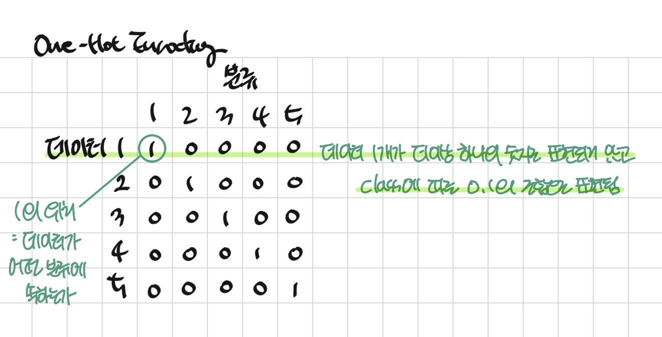
⭐ One-Hot Encoding 종류
1. sklearn: one_hot encoding
# sklearn: one_hot encoding

onehot_encoder=OneHotEncoder(sparse=False)
reshaped=y.reshape(len(y), 1)
onehot=onehot_encoder.fit_transform(reshaped)
print(onehot)
# [[1. 0. 0.]...[0. 0. 1.]]
print(onehot.shape) (150, 3)
2. keras: to_categorical
# keras: to_categorical

to_cat=to_categorical(y)
print(to_cat)
# [[1. 0. 0.]...[0. 0. 1.]]
print(to_cat.shape) (150, 3)
3. pandas: get_dummies
# pandas: get_dummies

print(pd.get_dummies(y))
[150 rows x 3 columns]
⚠️ One-Hot Encoding 후 발생한 타입 불일치 오류
ValueError: Classification metrics can't handle a mix of multilabel-indicator and continuous-multioutput targets
'''
y_test
[[1. 0. 0.]
 [0. 0. 1.]
 [1. 0. 0.]
 [0. 1. 0.]
 [0. 1. 0.]]

 y_predict
[[9.9925297e-01 7.4696867e-04 2.5099497e-13] 0
 [4.1013454e-10 2.7499644e-03 9.9725002e-01] 2
 [9.9945968e-01 5.4027850e-04 1.0871933e-13] 0
 [2.5293427e-06 6.0845017e-01 3.9154729e-01] 1
 [6.0919424e-06 8.0725497e-01 1.9273894e-01]] 1


Summary
y_test: [1. 0. 0.] 타입
y_predict: 실수 타입
(문제) 타입 불일치 오류
ValueError: Classification metrics can't handle a mix of multilabel-indicator and continuous-multioutput targets

(해결) y_predict = np.argmax(y_predict, axis=1)
argmax를 사용해서 arg 중 가장 큰 값을 뽑아 위치값을 반환

(최종 결과)
[0 2 0 2 1 1 0 2 0 2 2 2 2 0 0 0 2 0 2 1 0 2 1 1 0 2 1 1 1 2]
[0 2 0 1 1 1 0 2 0 2 2 2 2 0 0 0 2 0 2 1 0 2 1 1 0 2 1 1 1 1]
를 기준으로 accuracy 판단
'''
➕ fetch_covtype과 함께하는 One-Hot Encoding 응용
1. sklearn: one_hot encoding
문제1: ValueError: Expected 2D array, got 1D array instead: array=[5 5 2 ... 3]
OneHotEncoder는 Matrix 2차원만 입력받음
해결1: Matrix형태로 reshape → reshape: y = y.reshape(581012, 1)
문제2: TypeError: A sparse matrix was passed, but dense data is required.
train_test_splite를 사용할 수 있는 자료구조: numpy.ndarray
OneHotEncoding 후 자료구조: scipy.sparse._csr.csr_matrix
해결2: Use X.toarray() to convert to a dense numpy array.→ y = y.toarray()
# oneHotEncoder_fetch_covtype.py

import numpy as np

from tensorflow.keras.models import Sequential
from tensorflow.keras.layers import Dense

from sklearn.datasets import fetch_covtype
from sklearn.model_selection import train_test_split
from sklearn.preprocessing import OneHotEncoder
from sklearn.metrics import accuracy_score


# 1. Data
datasets = fetch_covtype()
x = datasets.data # (581012, 54)
y = datasets['target'] # (581012,)

y = y.reshape(581012, 1)
# 문제1: ValueError: Expected 2D array, got 1D array instead: array=[5 5 2 ... 3]
# OneHotEncoder는 Matrix 2차원만 입력받음
# 해결1: Matrix형태로 reshape → reshape: y = y.reshape(581012, 1)

ohe = OneHotEncoder()
ohe.fit(y)
y = ohe.transform(y)
print(type(y)) # <class 'scipy.sparse._csr.csr_matrix'>
y = y.toarray()
print(type(y)) # <class 'numpy.ndarray'>
# 문제2: TypeError: A sparse matrix was passed, but dense data is required.
# train_test_splite를 사용할 수 있는 자료구조: numpy.ndarray
# OneHotEncoding 후 자료구조: scipy.sparse._csr.csr_matrix
# 해결2: Use X.toarray() to convert to a dense numpy array.→ y = y.toarray()

x_train, x_test, y_train, y_test = train_test_split(
    x,y,
    shuffle=True,
    random_state=333,
    test_size=0.2,
    stratify=y
)


# 2. Model Construction
model = Sequential()
model.add(Dense(64, activation='relu', input_shape=(54, )))
model.add(Dense(64, activation='sigmoid'))
model.add(Dense(32,activation='relu'))
model.add(Dense(16,activation='linear'))
model.add(Dense(7,activation='softmax'))


# 3. Compile and train
model.compile(loss='categorical_crossentropy',
              optimizer='adam',
              metrics=['accuracy']
              )

model.fit(x_train, y_train, epochs=256, batch_size=128,
          validation_split=0.2,
          verbose=1)


# 4. evaluate and predict
loss, accuracy = model.evaluate(x_test, y_test)

y_predict = model.predict(x_test)
y_predict = np.argmax(y_predict, axis=1)
y_test = np.argmax(y_test, axis=1)

acc = accuracy_score(y_test, y_predict)
print("accuracy_score: ", acc)


'''
Result
loss:  0.596627414226532
accuracy:  0.7471494078636169
accuracy_score:  0.7471493851277505

'''
2. keras: to_categorical
문제: class 값이 0부터 시작하지 않으면 class 처음에 0 추가
해결: np.delete() 활용
# to_categorical_fetch_covtype.py

import numpy as np

from tensorflow.keras.models import Sequential
from tensorflow.keras.layers import Dense
from tensorflow.keras.utils import to_categorical

from sklearn.datasets import fetch_covtype
from sklearn.model_selection import train_test_split
from sklearn.metrics import accuracy_score

# 1. Data
datasets = fetch_covtype()
x = datasets.data
y = datasets['target']

y=to_categorical(y)
'''
print(type(y)) # 타입 확인 <class 'numpy.ndarray'>

문제
to_catergorical: class가 0부터 시작하지 않을 때, 앞에 0을 추가 -> 추가된 0만큼의 자원의 낭비가 발생
to_categorical(y): (0,1,2,3,4,5,6,7)
y: (1,2,3,4,5,6,7)

해결
y = np.delete(y, 0, 1)
np.delete(array, idx, axis)
열 -> 축(axis)이 지정되지 않으면 1차원으로 변환된(flatten) array에서 지정한 인덱스 값 제거
np.delete(a, 1, axis=1)과 같이 축을 지정: 축을 따라 지정한 인덱스의 서브어레이를 제거한 어레이를 반환

np.delete 참조:
numpy_delete.py

'''

y = np.delete(y, 0, axis=1)

x_train, x_test, y_train, y_test = train_test_split(
    x,y,
    shuffle=True,
    random_state=333,
    test_size=0.2,
    stratify=y
)


# 2. Model Construction
model = Sequential()
model.add(Dense(64, activation='relu', input_shape=(54, )))
model.add(Dense(64, activation='sigmoid'))
model.add(Dense(32,activation='relu'))
model.add(Dense(16,activation='linear'))
model.add(Dense(7,activation='softmax'))


# 3. Compile and train
model.compile(loss='categorical_crossentropy',
              optimizer='adam',
              metrics=['accuracy']
              )

model.fit(x_train, y_train, epochs=100, batch_size=128,
          validation_split=0.2,
          verbose=1)


# 4. evaluate and predict
loss, accuracy = model.evaluate(x_test, y_test)

y_predict = model.predict(x_test)
y_predict = np.argmax(y_predict, axis=1)
y_test = np.argmax(y_test, axis=1)

acc = accuracy_score(y_test, y_predict)
print("accuracy_score: ", acc)


'''
Result
accuracy_score:  0.729817646704474

'''
3. pandas: get_dummies
문제: type이 get_dummies 처리 후, (numpy → pandas) → value가 잘못 인식됨
해결: type 재변환: pandas → numpy
# get_dummies_fetch_covtype.py

import numpy as np
import pandas as pd

from tensorflow.keras.models import Sequential
from tensorflow.keras.layers import Dense

from sklearn.datasets import fetch_covtype
from sklearn.model_selection import train_test_split
from sklearn.metrics import accuracy_score


# 1. Data
datasets = fetch_covtype()
x = datasets.data
y = datasets['target']

y = pd.get_dummies(y)
'''
y = pd.get_dummies(y): idx 및 head 출력
부분 출력: print(y[:10])
print(y)
        1  2  3  4  5  6  7
0       0  0  0  0  1  0  0
1       0  0  0  0  1  0  0
2       0  1  0  0  0  0  0
3       0  1  0  0  0  0  0
4       0  0  0  0  1  0  0
...    .. .. .. .. .. .. ..
581007  0  0  1  0  0  0  0
581008  0  0  1  0  0  0  0
581009  0  0  1  0  0  0  0
581010  0  0  1  0  0  0  0
581011  0  0  1  0  0  0  0
[581012 rows x 7 columns]

print(type(y))
<class 'pandas.core.frame.DataFrame'>


Error
ValueError: Shape of passed values is (116203, 1), indices imply (116203, 7)
추가하고자 하는 값은 116203개의 값을 7개의 열에 추가해주려고 하는데, 정작 입력한 값은 116203개의 값을 1개의 열 값

Value가 잘못 인식된 이유:
get dummies를 통해서 y: (numpy-> pandas) -> np method에 pandas 바로 입력하면 해당 error 발생
해결: pandas -> numpy로 바꿔주기
'''

y = y.to_numpy() # pandas -> numpy
# y = y.values # pandas -> numpy

x_train, x_test, y_train, y_test = train_test_split(
    x,y,
    shuffle=True,
    random_state=333,
    test_size=0.2,
    stratify=y
)


# 2. Model Construction
model = Sequential()
model.add(Dense(64, activation='relu', input_shape=(54, )))
model.add(Dense(64, activation='sigmoid'))
model.add(Dense(32,activation='relu'))
model.add(Dense(16,activation='linear'))
model.add(Dense(7,activation='softmax'))


# 3. Compile and train
model.compile(loss='categorical_crossentropy',
              optimizer='adam',
              metrics=['accuracy']
              )

model.fit(x_train, y_train, epochs=256, batch_size=64,
          validation_split=0.2,
          verbose=1)


# 4. evaluate and predict
loss, accuracy = model.evaluate(x_test, y_test)

y_predict = model.predict(x_test)
y_predict = np.argmax(y_predict, axis=1)
y_test = np.argmax(y_test, axis=1)

acc = accuracy_score(y_test, y_predict)
print("accuracy_score: ", acc)


'''
Result
loss:  0.5851762294769287
accuracy:  0.7449549436569214
accuracy_score:  0.7449549495279812

'''
소스 코드
참고 자료
📑 원 핫 인코딩(One-Hot Encoding) 이해하기
📑 Numpy.Delete: How To Remove Elements From A NumPy Array
'Naver Clould with BitCamp > Aartificial Intelligence' 카테고리의 다른 글
| Classification Model Construction (0) | 2023.01.23 |
|---|---|
| Pandas pkg and Numpy pkg (1) | 2023.01.23 |
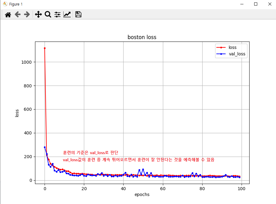
| Handling Overfitting: EarlyStopping (0) | 2023.01.22 |
| Validation Data (0) | 2023.01.22 |
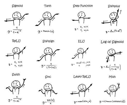
| Activation Function (0) | 2023.01.22 |