기본 환경: IDE: VS code, Language: Python
Model Construction 이후, 성능에 대한 판단 필요 → Model Performance Indicator
1. MAE: Mean Absolute Error, 평균 절대 오차
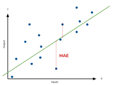
실제 값과 예측 값의 차이(실제 값 - 예측 값)를 절대값으로 변환 후 평균화
2. MSE: Mean Squared Error, 평균 제곱 오차
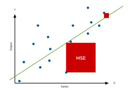
실제 값과 예측 값의 차이를 제곱 후 평균화
⭐ 데이터의 모형에 따른 MAE, MSE 선택
MAE
1. 이상치에 민감하지 않음
2. 데이터 모형의 범위가 크게 분산되어 있을 때 사용(과다 측정 예방)
MSE
1. 이상치에 민감함
2. 데이터 모형의 범위가 좁을 때 사용(과소 측정 보완)
⭐ Sequential Model의 mae, mse 지표 확인
# mae_and_mse.py
import numpy as np
from tensorflow.keras.models import Sequential
from tensorflow.keras.layers import Dense
from sklearn.model_selection import train_test_split
# 1. Data
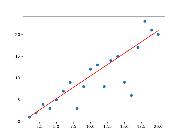
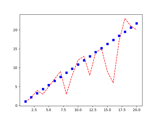
x = np.array(range(1,21))
y = np.array([1,2,4,3,5,7,9,3,8,12,13,8,14,15,9,6,17,23,21,20])
x_train, x_test, y_train, y_test = train_test_split(
x,y,
train_size=0.7,
shuffle=True,
random_state=123
)
# 2. Model Construction
model = Sequential()
model.add(Dense(64, input_dim=1))
model.add(Dense(32))
model.add(Dense(16))
model.add(Dense(1))
# 3. compile and train
model.compile(loss='mae', optimizer='adam', metrics=['mse']) # metrics를 활용한 여러 지표 확인
model.fit(x_train, y_train, epochs=128, batch_size=5)
# 4. Evalueate and Predict
loss = model.evaluate(x_test, y_test)
print("Loss: ", loss)
'''
# Result
mae: 3.0775
mse: 15.3362
'''
3. RMSE: Root MSE, 평균 오차
root(MSE)
⚠️ RMSE 지표는 Sequential 모델에서는 사용할 수 없는 지표이므로, 함수를 정의해서 사용
⭐ Sequential Model의 rmse 지표 확인
# rmse_def.py

import numpy as np

from tensorflow.keras.models import Sequential
from tensorflow.keras.layers import Dense

from sklearn.model_selection import train_test_split


# 1. Data
x = np.array(range(1,21))
y = np.array([1,2,4,3,5,7,9,3,8,12,13,8,14,15,9,6,17,23,21,20])

x_train, x_test, y_train, y_test = train_test_split(
    x,y,
    train_size=0.7,
    shuffle=True,
    random_state=123
)


# 2. Model Construction
model = Sequential()
model.add(Dense(64, input_dim=1))
model.add(Dense(32))
model.add(Dense(16))
model.add(Dense(1))


# 3. compile and train
model.compile(loss='mae', optimizer='adam', metrics=['mse'])
model.fit(x_train, y_train, epochs=128, batch_size=5)


# 4. Evalueate and Predict
loss = model.evaluate(x_test, y_test)
print("Loss: ", loss)

y_predict = model.predict(x_test)


from sklearn.metrics import mean_squared_error


def RMSE (y_test, y_predict):
    return np.sqrt(mean_squared_error(y_test, y_predict))
# def function_name(para1, para2):
    # return np.sqrt(mse), root(MSE)

print("RMSE: ", RMSE(y_test, y_predict))


'''
Result

MAE: 2.9459493160247803
MSE: 14.699475288391113
RMSE: 3.8339895717187855


'''
4. MSLE: Mean Squared Log Error, 평균 로그 오차
log(MSE)
5. MAPE: Mean Absolute Percentage Error, 평균 절대 비율 오차
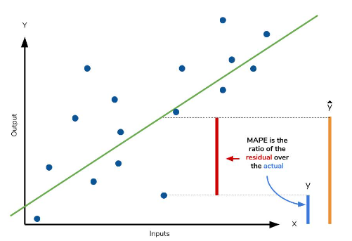
MAE*100%
6. MPE: Mean Percentage Error, 평균 비율 오차
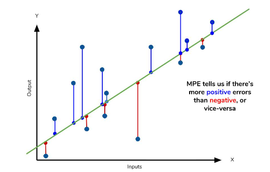
MAPE에서 절대값을 제외한 지표
모델이 실제값보다 낮은지 높은지 판단 가능
→ MAPE>0: 실제값>예측값
7. R2: R square, 결정 계수
회귀모형 내에서 설명변수 x로 설명할 수 있는 반응변수 y의 변동비율
총변동에서 설명 가능한 변동이 차지하는 비율
⚠️ 선형 관계에서 사용되는 지표이므로 2차 함수 등의 비선형 관계에서는 사용이 어려움
⭐ Sequential Model의 r2 지표 확인
# r2_score.py

import numpy as np

from tensorflow.keras.models import Sequential
from tensorflow.keras.layers import Dense

from sklearn.model_selection import train_test_split


# 1. Data
x = np.array(range(1,21))
y = np.array([1,2,4,3,5,7,9,3,8,12,13,8,14,15,9,6,17,23,21,20])

x_train, x_test, y_train, y_test = train_test_split(
    x,y,
    train_size=0.7,
    shuffle=True,
    random_state=123
)


# 2. Model Construction
model = Sequential()
model.add(Dense(64, input_dim=1))
model.add(Dense(32))
model.add(Dense(16))
model.add(Dense(1))


# 3. compile and train
model.compile(loss='mae', optimizer='adam', metrics=['mse'])
model.fit(x_train, y_train, epochs=128, batch_size=4)


# 4. Evalueate and Predict
loss = model.evaluate(x_test, y_test)
y_predict = model.predict(x_test)


from sklearn.metrics import mean_squared_error, r2_score # ','로 class 다중 삽입 가능


def RMSE (y_test, y_predict):
    return np.sqrt(mean_squared_error(y_test, y_predict))
print("RMSE: ", RMSE(y_test, y_predict))

r2 = r2_score(y_test, y_predict)
print("R: ", r2)


'''
Result for prediction

MAE: 3.0612
MSE: 15.1591
RMSE: 3.8482795786702315
-> loss: 낮을수록 고성능

R: 0.6485608399723322
-> accuracy: 높을수록 고성능

'''
➕ ScikitLearn Dataset을 이용한 예제
# indicator_with_california.py

import numpy as np

from tensorflow.keras.models import Sequential
from tensorflow.keras.layers import Dense

from sklearn.datasets import fetch_california_housing
from sklearn.model_selection import train_test_split


# 1. Data
datasets = fetch_california_housing()
x = datasets.data
y = datasets.target

x_train, x_test, y_train, y_test = train_test_split(
    x, y,
    train_size=0.7,
    random_state=123
)


# 2. model
model = Sequential()
model.add(Dense(64, input_dim=8))
model.add(Dense(32))
model.add(Dense(1))


# 3. compile and train
model.compile(loss='mae', optimizer = 'adam', metrics=['mse'])
model.fit(x_train, y_train, epochs=128, batch_size=64)


# 4. evaluate and predict
loss = model.evaluate(x_test, y_test)

y_predict = model.predict(x_test)


from sklearn.metrics import mean_squared_error, r2_score


def RMSE (y_test, y_predict):
    return np.sqrt(mean_squared_error(y_test, y_predict))
print("RMSE: ", RMSE(y_test, y_predict))

r2 = r2_score(y_test, y_predict)
print("R2: ", r2)


'''
Result

MAE: 0.6178
MSE: 0.8000
RMSE: 0.8944244298687739
R2: 0.39499231491934617
'''
8. Accuracy: 정확도
= (예측 결과가 동일한 데이터 건수/전체 예측 데이터 건수)
⚠️ 오차의 정도가 매우 낮음에도 불구하고 단순히 정오로만 판별하기 때문에 이진분류의 경우 정확도로만 평가하기에는 왜곡된 평가가 발생할 수 있으므로 보조 지표를 함께 사용해야 함
소스 코드
참고 자료
📑 [Scikit-learn] 회귀 모델 성능 측정 지표 : MAE, MSE, RMSE, MAPE, MPE
📑 Tutorial: Understanding Regression Error Metrics in Python
📑 [회귀분석] 결정계수(R²; Coefficient of Determination)
'Naver Clould with BitCamp > Aartificial Intelligence' 카테고리의 다른 글
| Pandas Package and Missing Value Handling (0) | 2023.01.21 |
|---|---|
| Environment Settings for GPU usage (0) | 2023.01.21 |
| Matplotlib: Scatter and plot (0) | 2023.01.21 |
| Split training data and test data (0) | 2023.01.21 |
| Scalar, Vector, Matirx, Tensor (0) | 2023.01.20 |