이모저모 개발 블로그

발생 Error

Git Bash에서 다음 명령어를 입력할 경우,

$ git push -u origin main
To https://github.com/HJ0216/TIL.git
 ! [rejected]        main -> main (fetch first)
error: failed to push some refs to 'https://github.com/HJ0216/TIL.git'

⭐ ! [rejected]        main -> main (fetch first)
⭐ error: failed to push some refs to 'https://github.com/HJ0216/TIL.git'

Error 발생

Error 원인

원격 저장소의 main branch에 저장되어있는 내용과 로컬 저장소의 내용이 일치하지 않아 발생

해결 방법

원격 저장소 내용을 로컬 저장소에 먼저 pull 시킴

$ git pull origin main
remote: Enumerating objects: 247, done.
remote: Counting objects: 100% (247/247), done.
remote: Compressing objects: 100% (187/187), done.
remote: Total 247 (delta 73), reused 157 (delta 38), pack-reused 0
Receiving objects: 100% (247/247), 59.49 KiB | 378.00 KiB/s, done.
Resolving deltas: 100% (73/73), done.
From https://github.com/HJ0216/TIL
 * branch            main       -> FETCH_HEAD
 * [new branch]      main       -> origin/main
fatal: refusing to merge unrelated histories

⚠️ 추가 문제: fatal: refusing to merge unrelated histories Error 발생

(참조: [해결 방법] fatal: refusing to merge unrelated histories)

참고 자료

📑[GitHub] Repository에 'main' branch로 push 하기

기본 환경: IDE: VS code, Language: Python

⭐ 서울시 따릉이 대여량 예측 경진대회 자료를 통한 Pandas pkg 및 결측치(Missing Value) 처리 방법

# dacon_seoul_ddarung.py
# dacon_seoul_ddarung data: https://dacon.io/competitions/open/235576/data

import numpy as np
import pandas as pd

from tensorflow.keras.models import Sequential
from tensorflow.keras.layers import Dense

from sklearn.model_selection import train_test_split
from sklearn.metrics import mean_squared_error


# 1. Data
path = './_data/ddarung/'
# 동일한 경로의 파일을 여러번 당겨올 경우, 변수를 지정해서 사용
# ./ = 현재 폴더
# _data/ = _data 폴더
# ddarung/ = ddarung 폴더

train_csv = pd.read_csv(path+'train.csv', index_col=0)
# path + 'train.csv': ./_data/ddarung/train.csv
# index_col을 입력하지 않을 경우 idx도 데이터로 인식하게 됨 (0번째 column은 data가 아닌 idx임을 안내)
# print(train_csv) [1459 rows x 11 columns] -> [1459 rows x 10 columns]

test_csv = pd.read_csv(path+'test.csv', index_col=0)
submission = pd.read_csv(path+'submission.csv', index_col=0)

print(train_csv.columns) # sklearn.feature_names

print(train_csv.info())
# null 값 제외 출력
# Int64Index: 715 entries, 총 데이터 수
# 결측치: 총 데이터 수 - Non-Null (수집못한 데이터)
print(test_csv.info()) # info -> null이 아닌 값(Non-Null) 출력
print(train_csv.describe()) # sklearn.DESC

# 결측치 처리 - '결측 데이터 제거'
print(train_csv.isnull().sum()) # data_set의 결측치(Null) 값 총계 출력
train_csv = train_csv.dropna() # pandas.dropna(): null 값을 포함한 데이터 행 삭제

x = train_csv.drop(['count'], axis=1)
# count column 삭제
# axis=0: index, axis: columns
print(x.shape) # [1459 rows x 9 columns] -> dropna로 인한 변경

y = train_csv['count']
print(y.shape)


x_train, x_test, y_train, y_test = train_test_split(
    x, y,
    shuffle=True,
    train_size=0.7,
    random_state=1234
)

print(x_train.shape, x_test.shape) #(1021, 9) (438, 9)
print(y_train.shape, y_test.shape) #(1021, ) (438, )


# 2. model
model = Sequential()
model.add(Dense(64, input_dim=9)) # input_dim = 9
model.add(Dense(64))
model.add(Dense(32))
model.add(Dense(16))
model.add(Dense(1)) # output_dim = 1


# 3. compile and train
model.compile(loss='mse', optimizer='adam') # RMSE가 평가지표이므로 유사한 mse 사용
model.fit(x_train, y_train, epochs=128, batch_size=32)


# 4. evaluate and predict
loss = model.evaluate(x_test, y_test)
print("Loss: ", loss)

y_predict = model.predict(x_test)
# test는 y값이 없으므로 train의 test dataset 사용


def RMSE (y_test, y_predict):
    return np.sqrt(mean_squared_error(y_test, y_predict))

rmse = RMSE(y_test, y_predict)
print("RMSE: ", rmse)


# for submission
y_submit = model.predict(test_csv) # predict() return numpy
submission['count'] = y_submit
# pandas(submission['count'])에 numpy(y_submit)를 직접 대입시키면 numpy가 pandas가 됨

submission.to_csv(path+'submission_230121.csv')



'''
Result

'''

⭐ Python Pandas 관련 유용한 Method 정리
pandas.read_cvs(): cvs file read
pandas.columns: column name

pandas.info(): null이 아닌 값(Non-Null) 출력
pandas.describe(): data description
pandas.isnull(): null 값 출력
pandas.dropna(): null data delete
pandas.drop(): column delete

⭐ Data Missing Value(결측치) 처리 방법
1. 삭제

 1.1. 결측치 데이터의 행 삭제

 1.2. 결측치 데이터의 열 삭제

2. 대체

 2.1. 이전 행 값으로 대체

 2.2. 다음 행 값으로 대체

 2.3. 원하는 값으로 대체

 2.4. 보간법으로 대체

→ method와 limit_direction에 따라 다르게 나타남

→ Data 값을 선형에 비례하는 값으로 결측값을 보간함

 2.5. 해당 열의 결측치를 제외한 평균값으로 대체

Pandas Dataset을 활용한 결측치 처리 예제

# missing_value_handling.py

import pandas as pd

dataset = pd.DataFrame([
    {'id': 1, 'val': None, 'pw': 2},
    {'id': 2, 'val': 21, 'pw': 3},
    {'id': 3, 'val': 19, 'pw': 0},
    {'id': 4, 'val': 24, 'pw': 1},
    {'id': None, 'val': 15, 'pw': 2},
    {'id': 5, 'val': 9, 'pw': 2},
    {'id': 6, 'val': 33, 'pw': 1},
    {'id': None, 'val': 40, 'pw': 2}
])

print(dataset)
'''
    id   val  pw
0  1.0   NaN   2
1  2.0  21.0   3
2  3.0  19.0   0
3  4.0  24.0   1
4  NaN  15.0   2
5  5.0   9.0   2
6  6.0  33.0   1
7  NaN  40.0   2
'''


# 1.1. 행 삭제
dataset_rev1 = dataset.dropna()
print(dataset_rev1)
'''
    id   val  pw
1  2.0  21.0   3
2  3.0  19.0   0
3  4.0  24.0   1
5  5.0   9.0   2
6  6.0  33.0   1
'''

# 1.2. 열 삭제
dataset_rev2 = dataset.dropna(axis='columns')
print(dataset_rev2)
'''
   pw
0   2
1   3
2   0
3   1
4   2
5   2
6   1
7   2
'''

# 2.1. 이전 행 값으로 대체
dataset_rev3 = dataset.fillna(method='pad')
print(dataset_rev3)
'''
    id   val  pw
0  1.0   NaN   2
1  2.0  21.0   3
2  3.0  19.0   0
3  4.0  24.0   1
4  4.0  15.0   2
5  5.0   9.0   2
6  6.0  33.0   1
7  6.0  40.0   2

이전 값이 없는 0번째 행은 NaN값 유지
'''

# 2.2. 다음 행 값으로 대체
dataset_rev4 = dataset.fillna(method='bfill')
print(dataset_rev4)
'''
    id   val  pw
0  1.0  21.0   2
1  2.0  21.0   3
2  3.0  19.0   0
3  4.0  24.0   1
4  5.0  15.0   2
5  5.0   9.0   2
6  6.0  33.0   1
7  NaN  40.0   2

다음 값이 없는 7번째 행은 NaN값 유지
'''

# 2.3. 원하는 값으로 대체
dataset_rev5 = dataset.fillna(0) # 0으로 대체
print(dataset_rev5)
'''
    id   val  pw
0  1.0   0.0   2
1  2.0  21.0   3
2  3.0  19.0   0
3  4.0  24.0   1
4  0.0  15.0   2
5  5.0   9.0   2
6  6.0  33.0   1
7  0.0  40.0   2
'''

# 2.4. 보간법으로 대체
dataset_rev6 = dataset.interpolate(method='linear',limit_direction='forward')
# 선형 비례 방법을 위에서부터 아래로 적용하여 NaN 값 채우기(0번째 행 제외)
dataset_rev6 = dataset.interpolate(method='linear',limit_direction='backward')
# 선형 비례 방법을 위에서부터 아래로 적용하여 NaN 값 채우기(7번째 행 제외)
print(dataset_rev6)
'''
forward
    id   val  pw
0  1.0   NaN   2
1  2.0  21.0   3
2  3.0  19.0   0
3  4.0  24.0   1
4  4.5  15.0   2
5  5.0   9.0   2
6  6.0  33.0   1
7  6.0  40.0   2

backward
    id   val  pw
0  1.0  21.0   2
1  2.0  21.0   3
2  3.0  19.0   0
3  4.0  24.0   1
4  4.5  15.0   2
5  5.0   9.0   2
6  6.0  33.0   1
7  NaN  40.0   2
'''

# 2.5. 결측치 값으로 제외한 평균값으로 대체
dataset_rev7 = dataset.fillna(dataset.mean())
print(dataset_rev7)
'''
    id   val  pw
0  1.0  23.0   2
1  2.0  21.0   3
2  3.0  19.0   0
3  4.0  24.0   1
4  3.5  15.0   2
5  5.0   9.0   2
6  6.0  33.0   1
7  3.5  40.0   2
'''

⭐ cvs 파일 관련 유용한 VS Code 확장자

: Excel Viewer, Rainbow CSV

소스 코드

🔗 HJ0216/TIL

참고 자료

📑 서울시 따릉이 대여량 예측 경진대회

📑 [pandas] 데이터 결측치 존재여부 확인 및 결측치 처리하기

📑 [Python pandas] 결측값 보간하기 (interpolation of missing values)

기본 환경: IDE:VS code, Language:Python

⭐ GPU 사용을 위한 환경 설정

1. Google: Nvdia Driver DownLoad

2. Google: Cuba DownLoad(v.11.4.4)

3. Google: cuDNN DownLoad

login(Sign in required)

Archived relaesae

Version에 맞는 cuDNN Download

4. D drive 내 'program' 폴더 생성
program 폴더 내에 해당 파일(다운로드 받은 파일 3개) 복사
(Ncvidia Driver) 527.56-desktop-win10-win11-64bit-international-dch-whql
(cuda) cuda_11.4.4_472.50_windows
(cuDNN) cudnn-11.4-windows-x64-v8.2.4.15

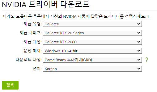
D drive -> 프로그램 폴더 내
4.1. (Nvidia Driver) 527.56-desktop-win10-win11-64bit-international-dch-whql 실행
→ driver만 설치, 사용자 정의 설치, 전체 설치

4.2. (cuda) cuda_11.4.4_472.50_windows
→ 동의 및 계속, 사용자 정의 설치
⚠️ Cuda 내 VS Integration 설치 제외, samples 설치 제외, Documentation 제외
GeForce 설치 제외
Component * 2 설치 제외

4.3. (cuDNN)cudnn-11.4-windows-x64-v8.2.4.15.zip
D drive에 zip 파일 풀기

4.4. C Drive -> 보기: 파일 확장명, 숨김 항목 표시 클릭
C:\Program Files\NVIDIA GPU Computing Toolkit\CUDA\v11.4
→ NVIDIA GPU Computing Toolkit\CUDA\v11.4 확인
⚠️ 가장 최신 버전의 CUDA가 아닌 가장 최근에 다운 받은 버전이 실행됨

4.5. D Drive에 담긴 프로그램 폴더 내 Cuda 폴더 내 파일 4개
(bin, include, lib, NVIDIA_SLA_cuDNN_Support.txt)를 
C:\Program Files\NVIDIA GPU Computing Toolkit\CUDA\v11.4에 복사해서 덮어쓰기

⭐ 설치 확인
cmd
nvidia-smi: 그래픽 드라이버 설치 확인
nvcc -V or nvcc --version : cuda ver 확인

⭐ GPU를 활용한 가상환경 만들기
anaconda prompt
conda create -n tf274gpu python=3.9.15 anaconda
conda env list: 가상환경 리스트 조회(⚠️ Base에서 확인)
activate tf274gpu
pip install tensorflow-gpu==2.7.4

VS code

Interpreter: 가상 환경 설정 tf274gpu 선택 후 Source Code 실행

# gpu_test.py

import tensorflow as tf
print(tf.__version__) # 2.7.4

gpus = tf.config.experimental.list_physical_devices('GPU')
# experimental: experimental method
# list_physical_devices 물리적인 장치 리스트
print(gpus)
# [PhysicalDevice(name='/physical_device:GPU:0', device_type='GPU')]
# Nvidia GPU만 출력됨(intel 내장형 GPU 출력 X)


if(gpus):
    print("GPU is running.")
else:
    print("GPU isn't running.")
# on GPU: GPU is running.
# on CPU: gpus=[], GPU isn't running.

gpus를 사용한 가상환경일 경우,

print(type(gpus)) # <class 'list'>

[PhysicalDevice(name='/physical_device:GPU:0', device_type='GPU')]

print(len(gpus)) = 1

-> 1개의 element가 있는 list 

비어있지 않은 리스트이므로 true 반환

그러므로 "GPU is running." 출력

⭐ Python에서의 boolean 기준

* list: 자료 구조 형태의 하나로 순서가 있는 수정가능한 객체의 집합

list = [1, 2, 3, 4, 5, 6, 7, 8, 9, 10]

* tuple: 자료 구조 형태의 하나로 순서가 있는 집합(수정 불가능)

tuple = (1, 2, 3, 4, 5)

소스 코드

🔗 HJ0216/TIL

참고 자료

📑 [Python] 리스트, 튜플

기본 환경: IDE: VS code, Language: Python

Model Construction 이후, 성능에 대한 판단 필요 → Model Performance Indicator

1. MAE: Mean Absolute Error, 평균 절대 오차

실제 값과 예측 값의 차이(실제 값 - 예측 값)를 절대값으로 변환 후 평균화

2. MSE: Mean Squared Error, 평균 제곱 오차

실제 값과 예측 값의 차이를 제곱 후 평균화

⭐ 데이터의 모형에 따른 MAE, MSE 선택
MAE
1. 이상치에 민감하지 않음
2. 데이터 모형의 범위가 크게 분산되어 있을 때 사용(과다 측정 예방)
MSE
1. 이상치에 민감함
2. 데이터 모형의 범위가 좁을 때 사용(과소 측정 보완)

⭐ Sequential Model의 mae, mse 지표 확인

# mae_and_mse.py

import numpy as np

from tensorflow.keras.models import Sequential
from tensorflow.keras.layers import Dense

from sklearn.model_selection import train_test_split


# 1. Data
x = np.array(range(1,21))
y = np.array([1,2,4,3,5,7,9,3,8,12,13,8,14,15,9,6,17,23,21,20])

x_train, x_test, y_train, y_test = train_test_split(
    x,y,
    train_size=0.7,
    shuffle=True,
    random_state=123
)


# 2. Model Construction
model = Sequential()
model.add(Dense(64, input_dim=1))
model.add(Dense(32))
model.add(Dense(16))
model.add(Dense(1))


# 3. compile and train
model.compile(loss='mae', optimizer='adam', metrics=['mse']) # metrics를 활용한 여러 지표 확인
model.fit(x_train, y_train, epochs=128, batch_size=5)


# 4. Evalueate and Predict
loss = model.evaluate(x_test, y_test)
print("Loss: ", loss)



'''
# Result

mae: 3.0775
mse: 15.3362

'''

3. RMSE: Root MSE, 평균 오차

root(MSE)

⚠️ RMSE 지표는 Sequential 모델에서는 사용할 수 없는 지표이므로, 함수를 정의해서 사용

⭐ Sequential Model의 rmse 지표 확인

# rmse_def.py

import numpy as np

from tensorflow.keras.models import Sequential
from tensorflow.keras.layers import Dense

from sklearn.model_selection import train_test_split


# 1. Data
x = np.array(range(1,21))
y = np.array([1,2,4,3,5,7,9,3,8,12,13,8,14,15,9,6,17,23,21,20])

x_train, x_test, y_train, y_test = train_test_split(
    x,y,
    train_size=0.7,
    shuffle=True,
    random_state=123
)


# 2. Model Construction
model = Sequential()
model.add(Dense(64, input_dim=1))
model.add(Dense(32))
model.add(Dense(16))
model.add(Dense(1))


# 3. compile and train
model.compile(loss='mae', optimizer='adam', metrics=['mse'])
model.fit(x_train, y_train, epochs=128, batch_size=5)


# 4. Evalueate and Predict
loss = model.evaluate(x_test, y_test)
print("Loss: ", loss)

y_predict = model.predict(x_test)


from sklearn.metrics import mean_squared_error


def RMSE (y_test, y_predict):
    return np.sqrt(mean_squared_error(y_test, y_predict))
# def function_name(para1, para2):
    # return np.sqrt(mse), root(MSE)

print("RMSE: ", RMSE(y_test, y_predict))



'''
Result

MAE: 2.9459493160247803
MSE: 14.699475288391113
RMSE: 3.8339895717187855


'''

4. MSLE: Mean Squared Log Error, 평균 로그 오차

log(MSE)

5. MAPE: Mean Absolute Percentage Error, 평균 절대 비율 오차

MAE*100%

6. MPE: Mean Percentage Error, 평균 비율 오차

MAPE에서 절대값을 제외한 지표

모델이 실제값보다 낮은지 높은지 판단 가능

→ MAPE>0: 실제값>예측값

7. R2: R square, 결정 계수

회귀모형 내에서 설명변수 x로 설명할 수 있는 반응변수 y의 변동비율
총변동에서 설명 가능한 변동이 차지하는 비율
⚠️ 선형 관계에서 사용되는 지표이므로 2차 함수 등의 비선형 관계에서는 사용이 어려움

⭐ Sequential Model의 r2 지표 확인

# r2_score.py

import numpy as np

from tensorflow.keras.models import Sequential
from tensorflow.keras.layers import Dense

from sklearn.model_selection import train_test_split


# 1. Data
x = np.array(range(1,21))
y = np.array([1,2,4,3,5,7,9,3,8,12,13,8,14,15,9,6,17,23,21,20])

x_train, x_test, y_train, y_test = train_test_split(
    x,y,
    train_size=0.7,
    shuffle=True,
    random_state=123
)


# 2. Model Construction
model = Sequential()
model.add(Dense(64, input_dim=1))
model.add(Dense(32))
model.add(Dense(16))
model.add(Dense(1))


# 3. compile and train
model.compile(loss='mae', optimizer='adam', metrics=['mse'])
model.fit(x_train, y_train, epochs=128, batch_size=4)


# 4. Evalueate and Predict
loss = model.evaluate(x_test, y_test)
y_predict = model.predict(x_test)


from sklearn.metrics import mean_squared_error, r2_score # ','로 class 다중 삽입 가능


def RMSE (y_test, y_predict):
    return np.sqrt(mean_squared_error(y_test, y_predict))
print("RMSE: ", RMSE(y_test, y_predict))

r2 = r2_score(y_test, y_predict)
print("R: ", r2)



'''
Result for prediction

MAE: 3.0612
MSE: 15.1591
RMSE: 3.8482795786702315
-> loss: 낮을수록 고성능

R: 0.6485608399723322
-> accuracy: 높을수록 고성능

'''

➕ ScikitLearn Dataset을 이용한 예제

# indicator_with_california.py

import numpy as np

from tensorflow.keras.models import Sequential
from tensorflow.keras.layers import Dense

from sklearn.datasets import fetch_california_housing
from sklearn.model_selection import train_test_split


# 1. Data
datasets = fetch_california_housing()
x = datasets.data
y = datasets.target

x_train, x_test, y_train, y_test = train_test_split(
    x, y,
    train_size=0.7,
    random_state=123
)


# 2. model
model = Sequential()
model.add(Dense(64, input_dim=8))
model.add(Dense(32))
model.add(Dense(1))


# 3. compile and train
model.compile(loss='mae', optimizer = 'adam', metrics=['mse'])
model.fit(x_train, y_train, epochs=128, batch_size=64)


# 4. evaluate and predict
loss = model.evaluate(x_test, y_test)

y_predict = model.predict(x_test)


from sklearn.metrics import mean_squared_error, r2_score


def RMSE (y_test, y_predict):
    return np.sqrt(mean_squared_error(y_test, y_predict))
print("RMSE: ", RMSE(y_test, y_predict))

r2 = r2_score(y_test, y_predict)
print("R2: ", r2)



'''
Result

MAE: 0.6178
MSE: 0.8000
RMSE: 0.8944244298687739
R2: 0.39499231491934617
'''

8. Accuracy: 정확도

= (예측 결과가 동일한 데이터 건수/전체 예측 데이터 건수)

⚠️ 오차의 정도가 매우 낮음에도 불구하고 단순히 정오로만 판별하기 때문에 이진분류의 경우 정확도로만 평가하기에는 왜곡된 평가가 발생할 수 있으므로 보조 지표를 함께 사용해야 함

소스 코드

🔗 HJ0216/TIL

참고 자료

📑 [Scikit-learn] 회귀 모델 성능 측정 지표 : MAE, MSE, RMSE, MAPE, MPE

📑 Tutorial: Understanding Regression Error Metrics in Python

📑 [회귀분석] 결정계수(R²; Coefficient of Determination)

기본 환경: IDE: VS code, Language: Python

Matplotlib을 활용한 데이터 시각화

기본적인 DNN 모델 구축 및 시각화를 통한 예측의 정확도 판별

# matplotlib_scatter_and_plot.py

import numpy as np

from tensorflow.keras.models import Sequential
from tensorflow.keras.layers import Dense

from sklearn.model_selection import train_test_split


# 1. Data
x = np.array(range(1,21))
y = np.array([1,2,4,3,5,7,9,3,8,12,13,8,14,15,9,6,17,23,21,20])

x_train, x_test, y_train, y_test = train_test_split(
    x,y,
    train_size=0.7,
    shuffle=True,
    random_state=123
)


# 2. Model Construction
model = Sequential()
model.add(Dense(64, input_dim=1))
model.add(Dense(32))
model.add(Dense(16))
model.add(Dense(1))


# 3. compile and train
model.compile(loss='mae', optimizer='adam')
model.fit(x_train, y_train, epochs=128, batch_size=4)


# 4. Evalueate and Predict
loss = model.evaluate(x_test, y_test) # 예측 전 평가

y_predict = model.predict(x) # training dataset을 predict에 사용
print("Result: ", y_predict)


import matplotlib.pyplot as plt

plt.scatter(x, y) # Scatter: 실제 x, y 데이터
plt.plot(x, y_predict, color="red") # plot: 실제 x, 예측 y 데이터
plt.show() # Scatter와 plot을 통해 시각적으로 예측을 비교, 분석할 수 있음



'''
Result

Epoch 128/128
4/4 [==============================] - 0s 5ms/step - loss: 1.9357

1/1 [==============================] - 0s 313ms/step - loss: 3.1006

Result:
[[ 1.0797057]
 [ 2.1201117]
 [ 3.160518 ]
 [ 4.2009234]
 [ 5.2413287]
 [ 6.2817335]
 [ 7.32214  ]
 [ 8.362547 ]
 [ 9.402951 ]
 [10.443358 ]
 [11.483764 ]
 [12.524168 ]
 [13.564573 ]
 [14.6049795]
 [15.645383 ]
 [16.685793 ]
 [17.7262   ]
 [18.766605 ]
 [19.807007 ]
 [20.847416 ]]
 
'''

plt.scatter(x, y): 파란색 점
plt.plot(x, y_predict, color="red"): 빨간색 실선

1. import matplotlib.pyplot as plt

matplotlib.pyplot library 함수를 사용하기 위해 import 후, 약칭 plt로 지정

2. plt.scatter(x, y)

실제 x, y 데이터를 scatter 함수에 대입하여, 산점도 반환

3. plt.plot(x, y_predict, color="red")

실제 x, 예측 y 데이터를 plot 함수에 대입하여, 예측 함수 반환

4. plt.show()

작성한 그래프 출력

➕ plot()

 - plot(y): plot 함수에 하나의 숫자 리스트가 대입될 경우, 해당 값을 y값으로 가정하고 x값 0, 1, 2 ...를 임의로 생성

 - plot(x,y): (x, y)에 대한 선형 함수 반환

 - plot(x1, y1, 'r--', x2, y2, 'bs'): (x1, y1)에 대한 빨간색 실선 및 (x2, y2)에 대한 파란색 네모 그래프 반환

→ 예시: (x, y) dataset과 (x, y_predict) dataset에 대한 그래프

# matplotlib_plot2.py

import numpy as np

from tensorflow.keras.models import Sequential
from tensorflow.keras.layers import Dense

from sklearn.model_selection import train_test_split


# 1. Data
x = np.array(range(1,21))
y = np.array([1,2,4,3,5,7,9,3,8,12,13,8,14,15,9,6,17,23,21,20])

x_train, x_test, y_train, y_test = train_test_split(
    x,y,
    train_size=0.7,
    shuffle=True,
    random_state=123
)


# 2. Model Construction
model = Sequential()
model.add(Dense(64, input_dim=1))
model.add(Dense(32))
model.add(Dense(16))
model.add(Dense(1))


# 3. compile and train
model.compile(loss='mae', optimizer='adam')
model.fit(x_train, y_train, epochs=128, batch_size=4)


# 4. Evalueate and Predict
loss = model.evaluate(x_test, y_test)
y_predict = model.predict(x)


import matplotlib.pyplot as plt

plt.plot(x, y, "r--", x, y_predict, "bs")
plt.show()

➕ load_digits를 활용한 이미지 반환

# matshow_load_digits.py

import matplotlib.pyplot as plt

from sklearn.datasets import load_digits
# 손글씨로 쓴 숫자를 분류하는 datasets


datasets = load_digits()
# print(datasets.shape) # numpy.shape, datasets=scikit learn

plt.gray() # 이미지의 기본색조: 회색조
plt.matshow(datasets.images[0]) # 훈련용 데이터 손글씨 0
plt.matshow(datasets.images[1]) # 훈련용 데이터 손글씨 1
# plt.matshow(): array -> image로 반환
plt.show()

소스 코드

🔗 HJ0216/TIL

참고 자료

📑 01. Matplotlib 기본 사용

📑 np.unique(y[Python] Python 20일차(예제로 배우는 파이썬 데이터 시각화)

📑 [Python] 10일차 - matplotlib, histogram 등